Quarto Basics
Introduction
This guide demonstrates how to create rich, interactive content using Quarto. Quarto is a powerful publishing system that allows you to combine narrative text, executable code, equations, figures, tables, and citations into beautiful documents.
Each section below includes:
- Code samples
- Rendered results showing what the output looks like
Let’s explore the main features you’ll need for academic and technical writing.
Text Formatting and Markdown Basics
Basic Text Formatting
Here are the fundamental text formatting options:
*italic text*,
**bold text**,
***bold italic text***
~~strikethrough text~~
`inline code`
superscript^2^, subscript~2~
Rendered result:
- italic text,
- bold text,
- bold italic text
strikethrough textinline code- superscript2, subscript2
Headings and Structure
# Main Heading (Level 1)
## Section Heading (Level 2)
### Subsection Heading (Level 3)
#### Sub-subsection Heading (Level 4)
Rendered result:
Main Heading (Level 1)
Section Heading (Level 2)
Subsection Heading (Level 3)
Sub-subsection Heading (Level 4)
Lists
Unordered Lists
* First item
  + Sub-item 1
  + Sub-item 2
    - Sub-sub-item
* Second item
Rendered result:
- First item
- Sub-item 1
- Sub-item 2
- Sub-sub-item
- Second item
Ordered Lists
1. First numbered item
2. Second numbered item
   i. Sub-item with roman numerals
   ii. Another sub-item
Rendered result:
- First numbered item
- Second numbered item
- Sub-item with roman numerals
- Another sub-item
Mathematical Equations
Inline Math
You can include mathematical expressions inline using single dollar signs:
$E = mc^2=> \(E = mc^2\)$\alpha + \beta = \gamma$=> \(\alpha + \beta = \gamma\).
Display Equations
For larger equations, use double dollar signs:
$$
\frac{\partial^2 u}{\partial t^2} = c^2 \nabla^2 u
$$ {#eq-wave}
Rendered result: \[ \frac{\partial^2 u}{\partial t^2} = c^2 \nabla^2 u \tag{1}\]
$$
P(X = k) = \frac{\lambda^k e^{-\lambda}}{k!}
$$ {#eq-poisson}
Rendered result: \[ P(X = k) = \frac{\lambda^k e^{-\lambda}}{k!} \tag{2}\]
Multi-line Equations
$$
\begin{align}
f(x) &= ax^2 + bx + c \\
f'(x) &= 2ax + b \\
f''(x) &= 2a
\end{align}
$$ {#eq-derivatives}
The {#eq-derivatives} is used to reference the equation in the text (see Cross-References).
Rendered result: \[ \begin{align} f(x) &= ax^2 + bx + c \\ f'(x) &= 2ax + b \\ f''(x) &= 2a \end{align} \tag{3}\]
Figures and Images
Static Images
You can include static images using markdown syntax:
{#fig-logo fig-alt="The Colib project logo" width="200px"}Rendered result:
Cross-References
How Cross-References Work
Quarto automatically generates numbered cross-references for:
- Equations: Use
eq-prefix (e.g.,#eq-wave) - Sections: Use
sec-prefix (e.g.,#sec-figures) - Figures: Use
fig-prefix (e.g.,#fig-logo) - Tables: Use
tbl-prefix (e.g.,#tbl-features)
Examples of Cross-References
- Reference an equation: "Using the wave equation (@eq-wave)..."
- Reference a section: "Details are provided in @sec-figures..."
- Reference a figure: "See @fig-logo for the Colib project logo..."
- Reference a table: "The results in @tbl-features indicate..."
Rendered result:
- Reference an equation: “Using the wave equation (Equation 1)…”
- Reference a section: “Details are provided in Section 5…”
- Reference a figure: “See Figure 1 for the Colib project logo…”
- Reference a table: “The results in Table 1 indicate…”
Citations and References
Citation Syntax
Quarto uses BibTeX for managing references. Citations are created using @ followed by the citation key:
Adding References
References should be stored in a .bib files and specified in the YAML header. You can specify multiple files by adding them to the bibliography list:
bibliography:
  - references.bib
  - references_2.bib
Example Bibliography Entry
@article{example2024,
  title={An Example Article},
  author={Smith, John and Doe, Jane},
  journal={Journal of Examples},
  volume={42},
  number={1},
  pages={1--10},
  year={2024},
  publisher={Example Press}
}
Advanced Features
Callout Blocks
Quarto provides several types of callout blocks:
:::{.callout-note}
This is a note callout. Use it for additional information.
:::

:::{.callout-tip}
This is a tip callout. Perfect for helpful suggestions.
:::

:::{.callout-warning}
This is a warning callout. Use for important caveats.
:::

:::{.callout-important}
This is an important callout. Use for critical information.
:::
Rendered result:
This is a note callout. Use it for additional information.
This is a tip callout. Perfect for helpful suggestions.
This is a warning callout. Use for important caveats.
This is an important callout. Use for critical information.
Source code
Use ``` to delimit blocks of source code and a language to syntax highlight code blocks.
Quarto can provide syntax highlighting for over 140 different languages (see the output of quarto pandoc --list-highlight-languages for a list of all of them).
```python
#| label: fig-polar
#| fig-cap: "A line plot on a polar axis"

import numpy as np
import matplotlib.pyplot as plt

r = np.arange(0, 2, 0.01)
theta = 2 * np.pi * r
```
Rendered result:
#| label: fig-polar
#| fig-cap: "A line plot on a polar axis"

import numpy as np
```python
#| label: fig-polar
#| fig-cap: "A line plot on a polar axis"

import numpy as np
import matplotlib.pyplot as plt

r = np.arange(0, 2, 0.01)
theta = 2 * np.pi * r
Code Blocks computation
Code blocks that use braces around the language name (e.g. ```{python}) are executable, and will be run by Quarto during render. Supported languages for execution are:
- Python
- R
- Julia
- Observable JS
You will find below a simple example. This example make use of the matplotlib and plotly Python packages to create a line plot on a polar axis, therefore they need to be installed before running the code block.
---
title: "matplotlib demo"
format:
  html:
    code-fold: true
jupyter: python3
---

For a demonstration of a line plot on a polar axis, see @fig-polar.

::: {#cell-fig-polar .cell execution_count=1}
``` {.python .cell-code}
import numpy as np
import matplotlib.pyplot as plt

r = np.arange(0, 2, 0.01)
theta = 2 * np.pi * r
fig, ax = plt.subplots(
  subplot_kw = {'projection': 'polar'}
)
ax.plot(theta, r)
ax.set_rticks([0.5, 1, 1.5, 2])
ax.grid(True)
plt.show()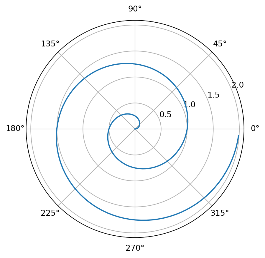
:::
Tables
Markdown Tables
You can create tables using markdown syntax:
| Feature | Supported | Notes |
|---------|-----------|-------|
| Code execution | ✓ | Python, R, Julia |
| Math equations | ✓ | LaTeX syntax |
| Cross-references | ✓ | Figures, tables, sections |
| Citations | ✓ | BibTeX format |
Rendered result:
| Feature | Supported | Notes |
|---|---|---|
| Code execution | ✓ | Python, R, Julia |
| Math equations | ✓ | LaTeX syntax |
| Cross-references | ✓ | Figures, tables, sections |
| Citations | ✓ | BibTeX format |
Tables from Code
Code sample:
#| label: tbl-data
#| tbl-cap: "Sample data analysis results"

import pandas as pd

# Create sample data
data = {
    'Method': ['Linear', 'Quadratic', 'Exponential', 'Logarithmic'],
    'R²': [0.65, 0.89, 0.94, 0.72],
    'RMSE': [2.3, 1.1, 0.8, 1.9],
    'Status': ['Fair', 'Good', 'Excellent', 'Good']
}

df = pd.DataFrame(data)
print(df.to_string(index=False))
Example output:
      Method   R²  RMSE    Status
      Linear 0.65   2.3      Fair
   Quadratic 0.89   1.1      Good
 Exponential 0.94   0.8 Excellent
 Logarithmic 0.72   1.9      Good