Underfrequency load shedding scheme based on System frequency response model
Underfrequency load shedding protection scheme based on System frequency response model
Context
System frequency response model (SFRM) is useful for representing frequency behavior of an electric power system after a sudden power imbalance occurs. It was developed to average the dynamic behavior of multiple synchronous machines into an equivalent single-generator unit model. It filters out all inter-generator oscillations and provides the average electric power system frequency response. SFRM was first introduced in [1] and was utilized in several publications since then.
UFLS is incorporated to SFRM as an additional feedback function (see Model description for more details). Apart from conventional UFLS algorithm, this model includes an innovative UFLS ([3], [4]) proposed by University of Ljubljana, Slovenia, with two different types of settings ( the shapes of tripping curves in f-M plane can be either L-shaped like in Fig. 5b (L-shaped) or ellipse-shaped like in Fig. 5c).
This model has been developed in the context of XX project which aims at studying the XX.
Model use, assumptions, validity domain and limitations
SFRM can be very handy for studying different frequency-control mechanisms, including Under-Frequency Load Shedding (UFLS), often referred to as Low-Frequency Demand Disconnection (LFDD). UFLS is governed by the system frequency and decreases system consumption once certain criteria are met. Depending on the criteria, a variety of UFLS algorithms exist in the literature [2], among which conventional frequency-threshold-based UFLS algorithm is prevailing. In the past, this type of system integrity protection scheme was rarely activated due to abundance of rotational masses, synchronized to the electrical power system. Namely, the so-called system inertia H has a stabilizing effect on electric-power frequency, making it very resilient to power imbalances. However, by replacing conventional generation with converter-interfaced sources without any rotational masses, system inertia is decreasing and as a result, the sensitivity to power imbalances is increasing. This calls for new frequency control and protection strategies, which can be easily studied using SFRM.
Most of the researchers agree that the flexibility of conventional UFLS is insufficient, especially under low-inertia conditions and uncertain stage sizes due to DER. Load disconnection based on frequency alone is simply inappropriate and offers poor adaptability. This is why numerous attempts can be found in the literature to increase UFLS adaptability to various operating conditions. One such innovation, developed at University of Ljubljana (noted as UL-UFLS) and presented in this model, takes advantage of frequency and its rate of change (rate-of-change-of-frequency - RoCoF) to add a second tripping criterion alongside frequency violation. Source [4] defines a frequency stability margin M(t), whose pros and cons were extensively discussed in [5], [6], [7], [8], [9].
Model description
System frequency response model
As illustrated in Fig. 1, the SFRM model consists of two transfer functions: TF1 represents a swing equation, providing mathematical formulation of a synchronous machine rotor motion, and TF2, covering a behavior of the speed governors and the turbines:
where:
- H is inertia constant in seconds,
- D is damping factor,
- Km is mechanical power gain factor,
- FH is a fraction of total power generated by the high-pressure turbine,
- TR is reheating time constant in seconds and
- R is a droop constant.
In Fig. 1, variables ΔP represent an initial power imbalance (usually a step-like function) and Pm power provided by governor control.
Underfrequency load shedding
UFLS is incorporated to SFRM as an additional feedback function providing PUFLS, as seen in Fig. 1. The impact of UFLS on acceleration power Pa is nonlinear, since UFLS provides discrete actions.
Apart from conventional UFLS algorithm, the model includes an innovative UFLS ([3], [4] intellectual property of University of Ljubljana, Slovenia), with two different types of settings.
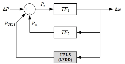
Fig.1. System frequency response model (SFRM) linear transfer function with non-linear UFLS (LFDD)
Conventional UFLS is designed to operate via activation of numerous frequency relays, scattered across several medium voltage substations (see Fig. 2). Triggering criteria is a violation of a frequency threshold setting fthr. The basic idea of conventional UFLS is to provide identical frequency threshold settings to selected groups of relays, making them act simultaneously. Each of these groups, containing relays from different locations in the network, is usually referred to as an UFLS stage. Most often, a transmission system operator (TSO) defines UFLS requirements, that are to be implemented by a distribution system operator (DSO). For the conventional UFLS, requirements are the following:
- number of stages (in Fig. 2 example equals 5),
- stage frequency thresholds,
- stage size (load decrease) and
- sum of all stage sizes.
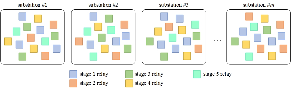
Fig.2. Frequency relay designation to UFLS stages
Appointment of relays that take part in each stage is a matter of DSO and so is the recurring period in which appointment is made. In practice, most of the conventional UFLS encompass up to 10 stages with frequency thresholds distributed evenly between 96% and 98% of the rated system frequency. Usually, relays are grouped into stages based on their average yearly power, yet increasing penetration of distributed energy resources (DER) dictates the need for more frequent (or even real-time) evaluation of appointments.
Additional tripping criterion
In order to increase UFLS adaptability to various operating conditions, this model embed a second tripping criterion alongside frequency violation as proposed by University of Ljublana. This second criterion takes advantage of frequency and its rate of change (rate-of-change-of-frequency - RoCoF) in this way:
where \(f_{set}\) is the frequency criterion in Hz and is defined differently for L-shaped tripping curve:
than for ellipse-shaped tripping curve:
where:
- \(M(t)\) is the instantaneous frequency Margin in seconds
- \(M_{set}\) is the frequency margin setpoint value in seconds
- \(f_{LIM}\) is the frequency limit in Hz
- \(f_{threshold}\) is the frequency threshold in Hz
Frequency stability margin
This new margin criterion aims at avoiding unnecessary shedding (overshedding) when the frequency is about to be stabilized by frequency control.
M(t) is defined as follows:
where:
- \(f(t)\) represents the instaneous frequency in Hz
- \(f_{LIM}\) is the frequency threshold in Hz
- \(RoCoF(t)\) is the rate-of-change-of-frequency in Hz/s
For understanding purposes, physical meaning of M(t) and its variation through time are represented graphically by Fig. 3. Fig. 3a depicts frequency response of an electric power system after negative power imbalance occurs at moment denoted with “event”, whereas M(t) at two instances M(t1) and M(t2) is shown in Fig. 3b.
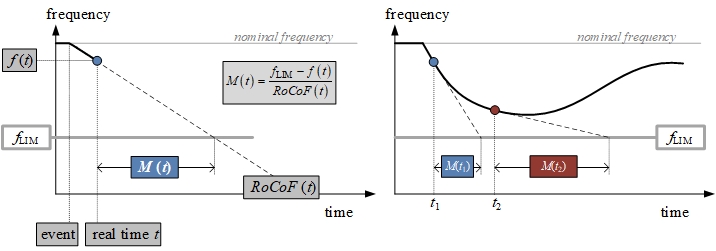
Fig.3. Graphical representation of frequency-stability margin M(t) calculation (a) and M(t) variation through time (b) after a negative power imbalance occurs
Frequency stability margin M(t) is transparently adopted to UFLS by depicting a trajectory of the operating point in the frequency f(t) versus frequency stability margin M(t) diagram (f-M plane). In Fig. 4a, several frequency response curves are depicted, among which red, black and blue are of interest. Red curve represents a stable case in which there is no need for UFLS activation. Black curve shows somewhat a borderline case in which frequency is indeed stabilized without UFLS, yet it reaches very low frequency values. A blue case is clearly unstable, meaning that UFLS activation is required. A corresponding three trajectories in f-M diagram are depicted in Fig. 4b, from which it is obvious that vicinity to lower-left hand side corner of the f-M diagram can be considered as a tripping criterion.
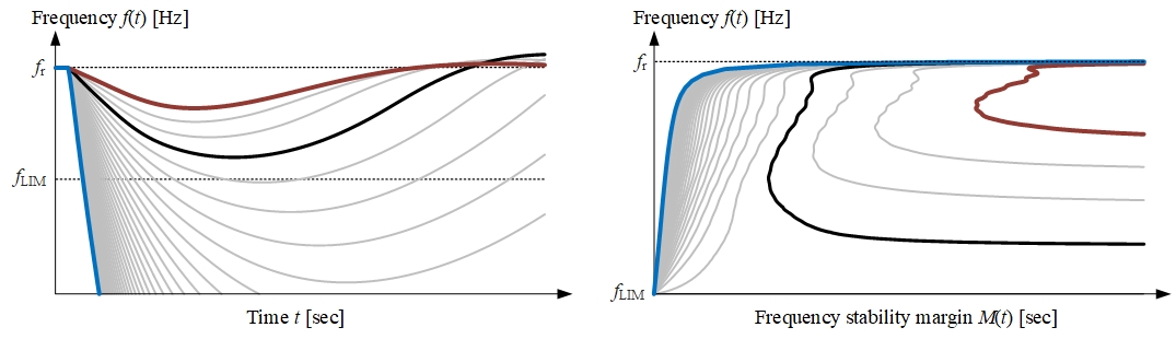
Fig.4. Different system frequency responses with respect to time (a) and corresponding trajectories in f-M plane (b)
One has numerous possibilities for defining the shape of tripping curves in f-M plane. In the presented use cases, we apply three of them, depicted in Fig. 5. Horizontal tripping lines in Fig. 5a correspond to M-independent conventional UFLS, whereas L-shaped (Fig. 5b) or ellipse-shaped (Fig. 5c) tripping curves indicate two possibilities, that we find most useful for practical applications.
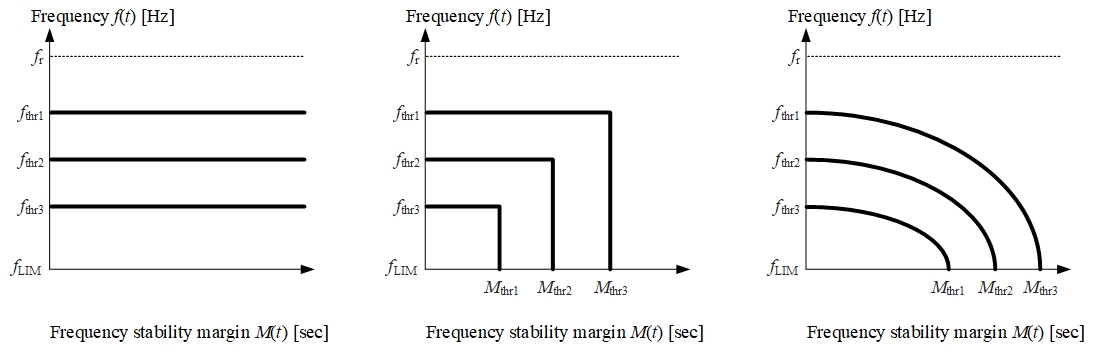
Fig.5. UFLS setting in f-M plane: conventional (a), L-shaped UL-UFLS (b), ellipse-shaped UL-UFLS (c)
Open Source Implementations
| Software | URL | Last consulted date |
|---|---|---|
| Python | Link | 03/06/2024 |
| Matlab/Simulink | Link | 03/06/2024 |
References
[1] P. M. Anderson and M. Mirheydar, ‘A low-order system frequency response model’, IEEE Trans. Power Syst., vol. 5, no. 3, pp. 720–729, Aug. 1990, doi: 10.1109/59.65898.
[2] T. Skrjanc, R. Mihalic, and U. Rudez, ‘A systematic literature review on under-frequency load shedding protection using clustering methods’, Renew. Sustain. Energy Rev., vol. 180, p. 113294, Jul. 2023, doi: 10.1016/j.rser.2023.113294.
[3] U. Rudež, ‘Method and device for improved under-frequency load shedding in electrical power systems: US 11 349 309 B2 - 2022-05-31’, 2022 [Online]. Available: https://si.espacenet.com/publicationDetails/originalDocument?FT=D&date=20220531&DB=&locale=si_SI&CC=US&NR=11349309B2&KC=B2&ND=4
[4] U. Rudez, D. Sodin, and R. Mihalic, ‘Estimating frequency stability margin for flexible under-frequency relay operation’, Electr. Power Syst. Res., vol. 194, p. 107116, May 2021, doi: 10.1016/j.epsr.2021.107116.
[5] U. Rudez and R. Mihalic, ‘RoCoF-based Improvement of Conventional Under-Frequency Load Shedding’, in 2019 IEEE Milan PowerTech, Jun. 2019, pp. 1–5. doi: 10.1109/PTC.2019.8810438.
[6] M. Vadillo, L. Sigrist, and U. Rudez, ‘Design and comparison of UFLS schemes of isolated power systems based on frequency stability margin’, in 2023 IEEE Belgrade PowerTech, Belgrade, Serbia: IEEE, Jun. 2023, pp. 1–6. doi: 10.1109/PowerTech55446.2023.10202842.
[7] U. Rudež, T. Dimitrovska, and R. Mihalič, ‘A RoCoF-based supplement to conventional under-frequency load shedding protection characteristic’, presented at the Pacworld 2019, Glasgow, Scotland: s. n.], p. Str. 1-12.
[8] D. Sodin, R. Ilievska, A. Čampa, M. Smolnikar, and U. Rudez, ‘Proving a Concept of Flexible Under-Frequency Load Shedding with Hardware-in-the-Loop Testing’, Energies, vol. 13, no. 14, Art. no. 14, Jan. 2020, doi: 10.3390/en13143607.
[9] A. Bonetti, J. Zakonjsek, and U. Rudez, ‘Bringing ROCOF into spotlight in Smart Grids: new standardization and UFLS method’, in 2020 2nd Global Power, Energy and Communication Conference (GPECOM), Oct. 2020, pp. 238–244. doi: 10.1109/GPECOM49333.2020.9248722.
Evaluate